Our first publication using Zooniverse data is now out in Nature Communications!

Read the original paper here. You can also check out Georgia's blog post on the Nature Ecology and Evolution community page here.

Physiological Requirements and Activity -- March 2021

by Asher Thompson

Animals’ physiological requirements are a driving factor in their behavior. Surface area to volume ratio (SA:V) can be a useful metric in understanding how animals will need to partition their time and activity in order to meet their physiological requirements and maintain homeothermy. Animals of larger mass have a smaller SA:V, so in warmer climates it is more difficult to stay cool because they have less surface area to lose heat through, and a greater volume which holds heat better. Many different methods of cooling have evolved such as sweating, panting, and increasing surface area through wrinkles or large ears, but all cooling methods result in water loss one way or another. Thus, hypothetically, smaller SA:V would be associated with greater water requirements and more activity at water sources.

My question was: is there a relationship between surface to volume ratio and African mammal activity at water pens?
To investigate this question, the camera trap dataset from this project was analyzed using R and RStudio to investigate the relationship between SA:V and animal activity at water pens. The activity metric used is the daily sum of total animals multiplied by the time spent at the water pen. Surface area values were calculated from each animal’s mass using a standard function and volume from the assumption that all animals have the same density with a 1:1 ratio of volume to mass. The SA:V and activity data were then analyzed considering treatment (dry site, filled pen, and drained pen) and season, tested for statistical significance, and the results were visualized.

A significant, inverse relationship was found between the log ratio of activity at the dry site versus filled or drained pen and SA:V values, and this relationship was seemingly consistent across the wet and dry seasons. The difference between dry and wet season does not seem to be significant, but further investigation is possible. This finding indicates that larger African mammals may aggregate more at surface water than smaller African mammals. As Earth’s climate increasingly changes, weather becomes more sporadic, and arid lands expand, understanding how animal’s behavior around water sources will be important for wildlife conservation strategies and domestic livestock management.

---

Carnivore Activity by Treatment -- March 2021

By Malik Elkouby

Standing water sources provide a critical resource to a wide range of savanna wildlife. While many camera trapping studies focus on herbivore activity around water sources, less is known about carnivore responses to changing water supply, due in part to the large sample size needed to determine behavioral patterns. Yet, due to their outsized effect on ecosystems, it is nonetheless important to understand how large mammalian carnivores respond to changing water availability, especially in the context of current climate change and increasing human draw-down of surface water.

I asked the question: How does experimental water removal affect carnivore activity? I hypothesized that carnivores would be spotted significantly less frequently at sites where water was experimentally removed (WPM) than at sites with water. I isolated the camera trap data for six carnivores including spotted hyenas, striped hyenas, cheetahs, jackals, leopards, and lions. I was able to plot the weekly trap sightings for each species across all three treatments (WPM, WPC, control).

I found that the results are not consistent across every species. Spotted hyenas, striped hyenas, and leopards actually had the higher sightings in the WPM treatment than in the WPC and control treatments. Cheetahs had nearly the same count for WPC and WPM, but were higher for the control treatment. Jackals and lions were the only ones that matched my hypothesis of carnivores being spotted more in WPC where water was present than in WPM where water was removed. However, the findings may be inaccurate since the sample size for each species was small.

---

Interspecies Contact Rates -- March 2021

By Viviana Martinez

The Earth’s climate is rapidly changing and its consequences can be seen across biomes as arid environments are expanding and water sources are depleting, potentially affecting the rate at which animals would return to watering holes. Because of this, I was interested in studying the relationship between temperature and interspecies contact rates at the watering holes. I was specifically interested in interspecies contact rates because this can give insight into community structure and reveal potential risks between trophic levels. Interspecies contacts were defined as the rate at which multiple species were observed during a specific time interval at each site.

Using the images from the camera traps, the temperature, date, and time were extracted using tesseract in R Studio. These values were then cross-referenced with those recorded from the field-loggers and historical records from the Nanyuki Airport Weather Station. After these values were checked, they were added to their corresponding observations from the camera traps. To conduct the first part of the analysis, I divided the dataset into time intervals with a five-minute buffer. I made the assumption that should 5+ minutes pass between the triggers, a new individual was responsible for that trigger. I then grouped each individual based on their assigned time interval, location, and treatment. I calculated the number of species observed per grouping and used this to find the interspecies contact rates, i.e. the groupings were used to find when multiple species were observed within a single lens at the sites. Using the groupings, I found the average temperature and contact rate per hour at each site.

Looking at average contact rates across all locations for each treatment type, we see that WPC had the greatest variation in contact rates throughout the day. The WPM treatment had some variation also following patterns corresponding with the hour (and consequently solar radiation), but they did not change at a rate as quickly as those at WPC. The CONT treatment had less variability throughout the day and had lower values for interspecies contact rates than the other two treatments on average.

Relating interspecies contact rates to temperature, again we can see how rate variation changed the most at WPC, with the maximum values occurring during periods of higher temperatures. From the analysis, the WPC treatment site had a significant effect on interspecies contact rates and there was a significant interaction between temperature and WPC sites with those rates. The CONT treatment had significantly fewer contacts than the other treatments. As predicted, there wasn't a significant effect of only temperature at CONT sites, but there was one at the other treatment sites. There was also a significant effect of the hour on those rates. The effect of hour on rates is not clear, but it may be due to light availability or influenced by the routine occurrence of domestic livestock, though this needs further investigation.

---

Joelle CantoAdams Results -- March 2021

Here is the link to my RStudio code to see how I visualized the data. The specific script is called "Joelle_Seasonality Script.R"

My question I used the camera data to answer was how the hour of watering hole visitations varies across the annual seasons between different herbivorous species? The animals I focused on were elephants, elands, impalas, plains zebras, water buffalo, and lions (as a predator reference). The months of the year were divided into "wet" and "dry" seasons based on historical data for the area; there are typically two dry and two wet seasons in a year. I specifically looked at the WPC Treatment, since those water pens at each location always had water, as well as the CONT Treatment that had no water as a control comparison. In the WPC water pen, the number of animals (mean_count) visiting watering holes significantly increased in the dry season, but the temporal niche between dry and wet season were not significantly different across the target species. If anything, the mode of the visiting hour each season shifted by an hour or so. In the continuous treatment, a significant number less animals visited the pens in either the wet or dry season compared to water pens, however its temporal niche followed a similar pattern to the water pens. Temporal niche does not seem to change across the seasons, but overall visitation increased in the dry season as expected, especially for water buffalo.

Hour of day was placed on a 12-hour circular scale centered at 6am (0). This was done because in Kenya there are about 12 light hours of the day (6am - 6pm) and 12 dark hours (6pm - 6am). Mean count of visit refers to the number of target species in each camera data point.

By location in both dry and wet season, plains zebras made up the bulk of visits throughout all times of the day. Looking at each animals visitations, there is a mixture of bimodal and unimodal distributions. Within each treatment, there is not much variation by season, but between treatments there is noticeable variation. This could also be due to the difference in the number of animals included for each treatment.

---

Results -- August 2020

We're starting to dig into the data a bit more, and have a cool preliminary plot to share!
As you may have noticed, many of the images you classify have a time stamp at the bottom. (You might have noticed that some of those seem wildly incorrect!) After a lot sleuthing, we were able to ensure that all of our images have the correct times in our analysis. We were curious about the daily distribution of times that different animal species were active. As you might have noticed, generally carnivores tend to be seen at night, and herbivores are seen during the day. Our new plot shows that relationship with amazing clarity:

(This is across all sites -- both water pans and our 'non-water' control sites. Also note that the scale is different for carnivores and herbivores for visualization purposes. There are roughly 20 herbivore triggers for every 1 carnivore trigger based on this plot, rather than a 1:1 relationship!)

However, you might ask: why on earth would carnivores choose to be active at night when there aren't any herbivores?
Well, one reason is that just because we don't catch herbivores on our camera triggers, it doesn't mean they aren't present! Many herbivores may rest or move to different locations at night. For example, impala tend to ruminate and lie down at night (and would be less likely to trigger cameras), and some zebras may move to more woody areas to avoid lions. Many carnivores (but not all!) have fairly good night-time eyesight, and, if prey are sleepy or have eyesight that is not well adapted to the dark, they may fare better in their quest for fare!
One question we plan to pursue is how different species use both water and non-water sites over the course of a day. Thanks to your help in making a robust dataset, we can start to ask and answer more sophisticated questions about animal behavior over time and space.

Stay tuned for more updates!

---

Results update -- May 2020

It's been a long time since we last shared some of our results! It's taken a while to get our pipeline established, but thanks to your help, we've managed to start some analyses!
Today we're sharing just a quick peek of animal responses to water manipulation.

There are a LOT of steps needed to go from our classifications to a final dataset in which we calculate a metric that represents animal abundance over time: daily animal-seconds. This number is the product of the number of animals present in the image, multiplied by the length of time for which the animal was present. This helps us to get an accurate measurement of exposure risk (rather than just counting occurrences, as animals are more likely to spend more time at water if it's there!).

Our experiment measures the change in animal aggregations at water in response to water draining and refilling. Below is a figure of animal-seconds for each of the six most common animals, split up by the type of site:

• Dry site: no water within 1km
• Filled site: water stayed filled for the whole experiment
• Drained site: water was drained "During" the experiment and refilled "Post" experiment.

As you can see, it looks like we see a pretty strong effect for elephants (red circle) and cattle. However, many of the other species don't seem to have changed their behavior very much in response to changing water supply. What's really cool is that this seems to match our data from dung counts. However, you'll notice that some of these error bars are really wide -- that's because animal movement is very variable, and we still need your help to get a better estimate of these values. In particular, we need quite a bit more data for our "Pre" and "Post" time points. We've just uploaded the last of these data, so we're in the final stretch!

Thanks for your interest in our project, and stay tuned for our next data update that will take a deeper dive into some of the less common species found in this project (carnivores, anyone?!)

---

Preliminary Results - Sneak Peek Dec 14

We're about a third of the way through this first round of IDs, and our dataset is growing daily. So far, you have classified many thousands of animals to help us better understand their watering hole usage.

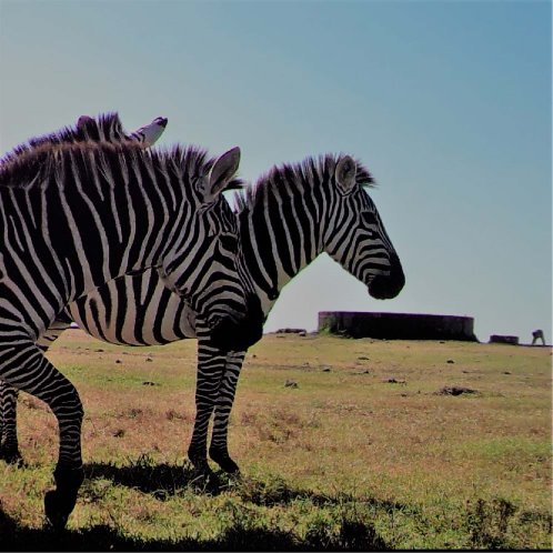
From the first two weeks of the project, a simple aggregation of the data shows that plains zebra and cattle are by far our most numerous species (which you probably could have guessed if you've been squinting at your computer counting those pesky cows!).

Here's a breakdown of what we have so far:

• Total Counts
  This is a graph that shows the total counts for each animal (using your average responses for each subject). As you can see, there are a couple of species that are super abundant, and quite a few that aren't too common. Keep in mind that this isn't a graph of the overall population of these animals, just the number of animals counted in the images here.
  ()

If we want to get a better idea of what's happening for the intermediate values, we can use a log scale for the y-axis:

• Subject Counts
  This graph shows the number of subjects by each species ID. This doesn't account for the number of animals in each photo. Comparing this graph to the graph above, you can see that elephants and zebra are in more photos than cattle are, but they are usually seen in much smaller groups, so that the total count of individuals is much greater for cattle.
  
  Note that this is also on a log scale

All of these preliminary results are just the start! We still have noisy data and need your IDs to help complete the project and to look at more complex patterns in the data! Thanks so much for your interest!